Data in the real world are often expensive, cluttered and limited by privacy rules. Synthetic data offers a solution – and they are already widely used:
- LLMS Train on AI-Generated Text
- Fraud systems simulate edge cases
- Vision models prior to fake images
SDV (Synthetic Data Vault) is an open source Python library that generates realistic tabular data using machine learning. It learns patterns from real data and creates high quality synthetic data for secure sharing, testing and modeling.
In this tutorial we use SDV to generate synthetic data step by step.
We first install the SDV Library:
from sdv.io.local import CSVHandler

connector = CSVHandler()
FOLDER_NAME = '.' # If the data is in the same directory

data = connector.read(folder_name=FOLDER_NAME)
salesDf = data['data']
Next, we import the necessary module and connect to our local folder that contains the data set files. This reads CSV files from the specified folder and saves them as Panda’s data frame. In this case we get access to the main data set using Data[‘data’].
from sdv.metadata import Metadata
metadata = Metadata.load_from_json('metadata.json')
We now import the metadata into our data set. This metadata is stored in a JSON file and tells SDV how to interpret your data. It includes:
- The Table Name
- The Primary key
- The Data type of each column (eg categorically, numeric, datetime, etc.)
- Optional Column formats Like Datetime -The patterns or ID -patterns
- Table Relationship (for Multi-Table Setups)
Here is a trial metadata.json format:
{
  "METADATA_SPEC_VERSION": "V1",
  "tables": {
    "your_table_name": {
      "primary_key": "your_primary_key_column",
      "columns": {
        "your_primary_key_column": { "sdtype": "id", "regex_format": "T[0-9]{6}" },
        "date_column": { "sdtype": "datetime", "datetime_format": "%d-%m-%Y" },
        "category_column": { "sdtype": "categorical" },
        "numeric_column": { "sdtype": "numerical" }
      },
      "column_relationships": []
    }
  }
}
from sdv.metadata import Metadata
metadata = Metadata.detect_from_dataframes(data)Alternatively, we can use the SDV library to automatically derive the metadata. However, the results may not always be accurate or complete, so you may need to review and update it if there are any discrepancies.
from sdv.single_table import GaussianCopulaSynthesizer

synthesizer = GaussianCopulaSynthesizer(metadata)
synthesizer.fit(data=salesDf)
synthetic_data = synthesizer.sample(num_rows=10000)
With the metadata and the original data set ready, we can now use SDV to train a model and generate synthetic data. The model learns the structure and patterns of your real data set and uses this knowledge to create synthetic items.
You can check how many rows to be generated using Num_rows argument.
from sdv.evaluation.single_table import evaluate_quality

quality_report = evaluate_quality(
    salesDf,
    synthetic_data,
    metadata)
The SDV library also provides tools to evaluate the quality of your synthetic data by comparing them to the original data set. A good place to start is by generating one Quality report
You can also visualize how the synthetic data is compared to the real data using SDV’s built -in planning tools. For example, imports get_column_plot from sdv.evaluation.single_table To create comparison charts for specific columns:
from sdv.evaluation.single_table import get_column_plot

fig = get_column_plot(
    real_data=salesDf,
    synthetic_data=synthetic_data,
    column_name="Sales",
    metadata=metadata
)

fig.show()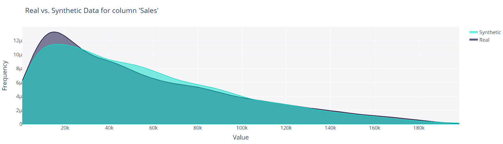
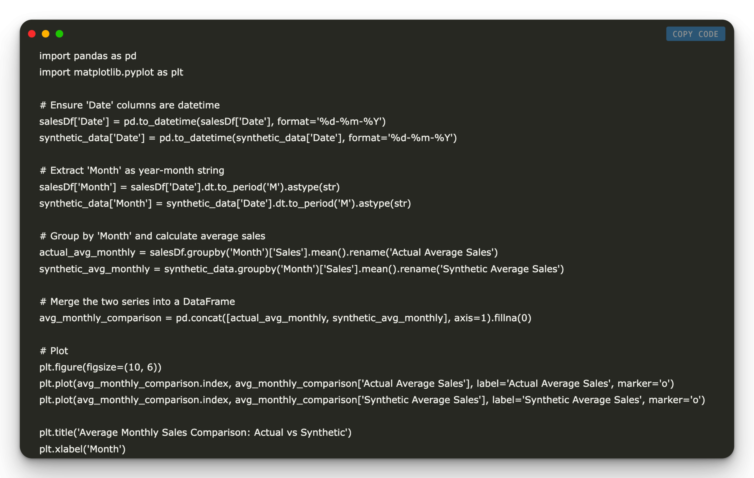
We can observe that the distribution of the ‘Sales’ column in the real and synthetic data is very similar. To explore further, we can use Matplotlib to create more detailed comparisons – such as visualizing the average monthly sales trends across both data sets.
import pandas as pd
import matplotlib.pyplot as plt

# Ensure 'Date' columns are datetime
salesDf['Date'] = pd.to_datetime(salesDf['Date'], format="%d-%m-%Y")
synthetic_data['Date'] = pd.to_datetime(synthetic_data['Date'], format="%d-%m-%Y")

# Extract 'Month' as year-month string
salesDf['Month'] = salesDf['Date'].dt.to_period('M').astype(str)
synthetic_data['Month'] = synthetic_data['Date'].dt.to_period('M').astype(str)

# Group by 'Month' and calculate average sales
actual_avg_monthly = salesDf.groupby('Month')['Sales'].mean().rename('Actual Average Sales')
synthetic_avg_monthly = synthetic_data.groupby('Month')['Sales'].mean().rename('Synthetic Average Sales')

# Merge the two series into a DataFrame
avg_monthly_comparison = pd.concat([actual_avg_monthly, synthetic_avg_monthly], axis=1).fillna(0)

# Plot
plt.figure(figsize=(10, 6))
plt.plot(avg_monthly_comparison.index, avg_monthly_comparison['Actual Average Sales'], label="Actual Average Sales", marker="o")
plt.plot(avg_monthly_comparison.index, avg_monthly_comparison['Synthetic Average Sales'], label="Synthetic Average Sales", marker="o")

plt.title('Average Monthly Sales Comparison: Actual vs Synthetic')
plt.xlabel('Month')
plt.ylabel('Average Sales')
plt.xticks(rotation=45)
plt.grid(True)
plt.legend()
plt.ylim(bottom=0)  # y-axis starts at 0
plt.tight_layout()
plt.show()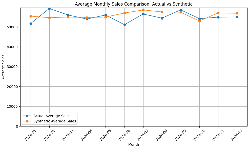
This diagram also shows that the average monthly sale in both data sets is very similar with only minimal differences.
In this tutorial, we demonstrated how to prepare your data and metadata for synthetic data rating using the SDV library. By training a model on your original data set, SDV can create high quality synthetic data that closely reflects the real data patterns and distributions. We also explored how to evaluate and visualize the synthetic data, confirming that key metrics as sales distributions and monthly trends remain uniform. Synthetic data offers a powerful way of overcoming privacy and accessibility challenges while allowing robust data analysis and machine learning work.
Check the laptop on GitHub. All credit for this research goes to the researchers in this project. You are also welcome to follow us on Twitter And don’t forget to join our 95k+ ml subbreddit and subscribe to Our newsletter.

I am a candidate for a civil engineer (2022) from Jamia Millia Islamia, New Delhi, and I have a great interest in data sciences, especially neural networks and their use in different areas.